 |
Understanding
the Edge-Driven Convection Hypothesis
|
 |
Introduction
Edge Driven Convection
(EDC) is an instability that occurs at the boundary
between thick stable lithosphere (for example, an
Archean craton) and thinner lithosphere (King
& Anderson,
1998; King
& Ritsema,
2000). Elder (1976) first discussed the
effect of flow near a stationary continent drawing
on the results of laboratory experiments. Vogt
(1991) proposed that a pair of asthenospheric upwellings,
paralleling and controlled by the temperature contrast
across the North American continental margin were
responsible for formation of the Bermuda and Labrador
rises. King
& Ritsema
(2000) present images from a seismic tomography
model that are consistent with the down-welling limbs
of the EDC instability associated with cratonic roots
under Africa. These examples appeal to a small-scale
instability driven by lateral variations in temperature
near the top of the mantle (Anderson,
2001).
The vertical cross
section through the tomographic model S20RTS (Ritsema
et al.,
1999) across the south-central Atlantic has been
interpreted by King
& Ritsema
(2000) as downwelling limbs under the Atlantic
side of the African and South American cratons (Figure
1). The saturated blue region in the upper 100 km
is 4% faster than PREM while the blue limbs, which
extend to 500 km depth, are interpreted as the down-going
limbs of the EDC instability. Because of ray focusing
and dispersion, it may be easier to image the cold,
fast, down-going limbs of the EDC flow than the warmer,
upwelling part of the EDC flow that we expect to find
beneath hotspots. A corollary of this is that seismic
experiments testing the EDC flow hypothesis should
have a distribution of stations covering not only
the hotspot under investigation, but also the potential
“edge”.
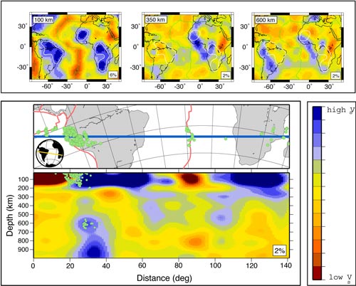
Figure 1: A vertical cross-section
through the tomographic model S20RTS. Velocity anomalies
are referenced to PREM. Blue regions represent anomalies
larger (faster) than PREM and red represent regions
smaller (slower) than PREM. The scale is ±
2%. (Adapted from King
& Ritsema, 2000).
EDC requires a stable, thick continental
or cratonic root adjacent to a thinner (probably oceanic)
plate. Because of our limited knowledge of the thermal,
mechanical and chemical properties of the cratonic
root, it is difficult to place a bound on the minimum
thickness root necessary to generate an EDC instability.
While not exhausting parameter space, our numerical
experiments suggest that a 150 km thick craton/root
is the minimum required.
Seismic evidence supports the existence
of such roots under thick cratons (e.g., Sipkin
& Jordan, 1975; Ritsema
et al.,
1999). The lack of correlation between the long-wavelength
geoid and continents (Kaula, 1967; Shapiro
et al., 1999a) indicates that continental roots
are not simply structures formed by prolonged conductive
cooling and must be compositionally distinct from
the upper mantle. The long-term stability of these
roots is assumed in the EDC hypothesis; however EDC
is not related to the “delamination” of
the continental root. The stability of thermo-chemical
continental roots is a different problem that has
been examined by Shapiro et al. (1999b).
What is the physical
mechanism behind EDC?
EDC is driven by the vertical temperature
variation along the “edge” (boundary) of
the cratonic root. Because the craton and the cratonic
root are assumed to have been stable for a billion years
or more, we assume that the root is not significantly
deforming and that from the point of view of the mantle,
this root is a stable, fixed boundary. This is not to
say that there is not a small amount of erosion of the
cratonic root during this process, but including this
effect is computationally challenging and introduces
a new set of issues to be considered including the strength
and composition of the cratonic root. Therefore we begin
with the fairly simple assumption that the cratonic
root is a rigid and undeforming boundary. Because the
craton and oceanic lithosphere are stable, fixed boundaries
and the mantle is mobile, this configuration will evolve
to a point where the base of the craton and the base
of the oceanic plate are at nearly the same temperature.
As a result, the temperature along the near-vertical
craton boundary will be almost uniform. This vertical-wall
boundary is an unstable condition and will generate
small-scale flow (Figure 2).
Figure 2: Cartoon illustrating the
small-scale convective flow field from the EDC instability
along a craton boundary. The EDC instability is driven
by the temperature discontinuity at the vertical wall
separating the cold, stable craton from the warmer asthenosphere
(King
& Anderson, 1998).
The arrows in the cartoon illustrate
the resulting flow pattern in the absence of other upper-mantle
instabilities or large-scale plate flow. This is similar
to the flow pattern that forms deep-water masses at
the edges of the polar ice shelves. (The deep-water-mass
formation problem is more complex because the freezing
and melting of seawater affects not only the temperature
but also the salinity of the water.) Because this is
a short-wavelength flow pattern, the endothermic 660-km
phase transformation acts as an efficient barrier to
the flow (Tackley, 1996). Given the nature
of convective instabilities (Turcotte & Schubert,
1982), the flow would naturally adopt a horizontal wavelength
similar to (i.e., 1-1.5 times) the depth (~
600 km). Therefore it is reasonable to expect that weak
upwellings 600-1,000 km from the craton boundary result
from EDC.
The EDC calculations illustrated below
are computed using a compressible convection formulation
for a two-dimensional Cartesian geometry (Figures 3
& 4). These represent our attempt at the most realistic
parameters for the upper mantle. The calculations are
performed in a 2,890 by 2,890 km domain with 256 bilinear
elements in each direction, although only a subregion
of the domain is shown. The Rayleigh number used is
2.5 x 10⁷, a reasonable approximation for
Earth. The parameters are chosen so that the resulting
surface heat flow approximates the mean surface heat
flow of Earth. The initial thermal structure of an ocean
basin is calculated using the solution for a moving
plate, while the thermal structure of the cratonic lithosphere
is calculated using the half-space solution and assuming
that the craton is uniformly 500 Ma.
|
|
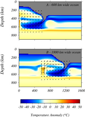
Figure 3: Temperature
anomalies (adiabatic temperature profile removed)
and velocity fields from calculations with a step
change in lithospheric thickness. The width of
the ocean basin (thin lithosphere) is 600 (A)
and 1,800 km (B). In each calculation, the width
of the ocean basin is fixed through time. Both
panels are taken 50 Myr after the initial condition. |
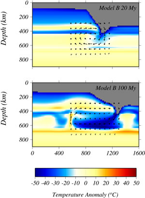
Figure 4: Temperature
anomalies (adiabatic temperature profile removed)
and velocity fields from calculations with a step
change in lithospheric thickness. The width of
the ocean basin (thin lithosphere) is 1,800 km.
The temporal evolution of the calculation Model
B above is shown in panels above. The top is 20
Myr after the initial condition, the lower is
100 Myr after the initial condition. |
No attempt has been made to address
the composition of the craton at this point. The cratonic
root is assumed to be highly viscous and neutrally buoyant
as required for cratonic root stability (e.g., Shapiro
et al., 1999a; Lenardic & Moresi,
1999). The calculations also contains solid-solid phase
transformations at 410 and 660 km depth, which confine
EDC to the upper mantle. The Clapeyron slopes used for
these phase changes are 3.5 K/MPa (at 410 km) and -2.8
K/MPa (at 700 km), consistent with the values of the
olivine to wadsleyite phase transformation (at about
410 km) and the ringwoodite to perovskite plus magnesiowüstite
phase transformation (at about 660 km). There is an
additional factor of 30 increase in viscosity at 700
km depth. This viscosity profile is consistent with
many geophysical estimates of mantle rheology. The viscosity
of the fluid depends on pressure and temperature, but
not stress, following the creep properties of olivine.
The location of the craton with respect
to the edges of the computational domain is fixed in
each calculation. The distance between the edge of the
craton and the ocean ridge is varied from 400 to 1,600
km in a series of calculations to study the pattern
of the small-scale flow as the width of the ocean basin
is increased. When the ocean basin is narrow (Model
A, Figure 3 top), an upwelling forms along the edge
of the computational domain, which represents the central
spreading axis of the ocean basin. A downwelling forms
beneath the craton, slightly craton-ward of the craton-ocean
margin. As the width of the ocean basin increases with
time (Model B, Figure 3 bottom), the upwelling moves
off the spreading axis while the downwelling remains
fixed with respect to the craton-ocean boundary. The
resulting EDC cell is at most 800-1,000 km wide regardless
of the location of the craton. EDC reaches a peak velocity
of about 30 mm/yr after about 80-100 Myr. After 100
Myr the vigor of the flow slowly decreases (compare
Figure 4 top (20 Myr) and bottom (100 Myr)).
When applying the EDC hypothesis to
specific cases, it is important to consider that the
EDC instability is relatively weak and can be overwhelmed
by flow due to other temperature anomalies in the upper
mantle, relative motion between the craton and upper
mantle, or general plate-scale flow (c.f., King
& Anderson,
1998). This might explain why hotspots could be
associated with the African cratons via EDC, as suggested
by King
& Ritsema
(2000), while at the same time similar features
(hotspots or upper-mantle seismic anomalies) are not
observed at most other cratons. The African cratons
are ideal for EDC because they are far from subduction
zones and other “active” features of mantle
flow and may be relatively stationary with respect to
the upper mantle.
Effects
of continents and cratons that can lead to small-scale
convection yet differ from EDC
Supercontinent Insulation
There have been a number of suggestions
that (super)continents may effectively “insulate”
the upper mantle, leading to a buildup of heat (Gurnis,
1988; Anderson, 1994; Lowman & Jarvis,
1995; 1996). This lateral variation in temperature between
the warm, insulated mantle beneath the (super)continent
and “normal” upper mantle can drive an upper-mantle
convective flow pattern. This continental insulation
flow, is not the same as the EDC flow pattern described
above, although it is the primary source of buoyancy
driving the convective flow pattern seen in the calculations
presented by King & Anderson (1995). With
continental-insulation flow, the upper mantle beneath
the continental lithosphere is hotter than the upper
mantle beneath the oceanic lithosphere.
The pattern of flow resulting from
continental insulation is opposite to that of EDC flow
(Figure 5). In addition, the wavelength of this flow
depends on the wavelength of the upper mantle temperature
anomalies. Thus, continental insulation temperature
anomalies can be much broader than those associated
with EDC but, they not likely to form beneath isolated
cratons or even small continents. Anderson
(1982, 1998) suggests that continental insulation can
increase the upper mantle temperature by as much as
200°C. Based on our simple modeling (King &
Anderson, 1995, 1998)
a large-scale, 200°C anomaly would drive a major
upper mantle convection cell and would most likely wipe
out any EDC effects. At the initial stages of rifting
of a continent, upwelling should occur as warm mantle
from beneath the continent occupies the space created
by the spreading continental masses. The active rifting
will dominate until the “edges” develop.
EDC flow could develop once the continental or cratonic
“edge” has migrated some distance from the
forming rift.
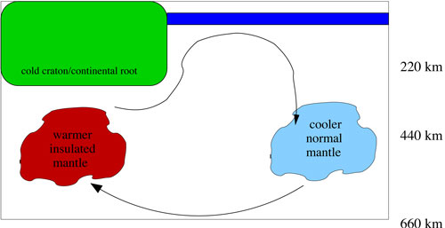
Figure 5: A cartoon illustrating
the small-scale convective flow field resulting from
lateral temperature anomalies in the upper mantle due
to continental insulation (c.f., King & Anderson,
1995).
In continental-insulation-driven
flow, hot material from beneath the craton flows
upward along the craton boundary. From simple
numerical modeling, King
& Anderson
(1998) suggest that lateral temperature variations
under a continent in excess of 30°C are required
for continental-insultation flow to significantly
modify (or even shut off) EDC flow. Comparing
the calculations in Figure 6, the top calculation
(A) is dominated by the large-scale mantle flow
(75°C hotter under the continent and 75°C
colder under the oceanic plate). In calculation
(B), one can just make out a small counter-flow
that forms to the “ocean-side” of
the thick “cratonic” boundary layer.
(Arrows are shown only at every fourth point for
clarity.) In calculation (C) the large-scale mantle
flow is small and the arrows indicate EDC flow
around the lithospheric discontinuity.
These calculations illustrate
the fragility of the EDC instability. In the presence
of other anomalies in the upper mantle, the EDC
instability can be overwhelmed. In other numerical
experiments, King
& Anderson (1998,
Figure 3b) show that if the craton is moving
relative to the upper mantle beneath it, at speeds
greater than 2 cm/yr, the shear flow between the
mantle and the craton is enough to suppress the
EDC instability.
Figure 6: Three calculations
where a sinusoidal mantle temperature perturbation
was added to an otherwise isothermal mantle beneath
the boundary layer structure illustrated by the
isotherms (see Figure 3). The size of the mantle
temperature perturbation was varied from about
3°C to 150°C. |
|
It is important to point out that continental
insulation may be a rather unusual situation, requiring
large continental areas (supercontinents) that are stable
for a long period of time. Lowman & Jarvis
(1996) suggest that rather than thermal insulation,
the mechanism for warm upper mantle beneath large supercontinents
may be upwelling “return” flow beneath the
continent resulting from subduction which often surrounds
supercontinents. It is possible that the upper mantle
beneath the former Pangea is still warmer than average,
with some effect from “insulation” the continent.
Lithospheric Delamination
Finally, lithospheric delamination
could also generate an upper mantle scale flow. It is
difficult to maintain a deep continental root in convective
models (c.f., Shapiro et al., 1999b) although
one can argue that the geophysical evidence suggests
their stability is less difficult for the Earth than
it is for numerical modelers. Progress is slowly being
made (e.g., Shapiro et al., 1999a; Lenardic
& Moresi, 1999; Lenardic et al., 2003).
The flow generated by lithospheric delamination is illustrated
in Figure 7. I include this case primarily to illustrate
that EDC and lithospheric delamination are different.
(See also Lithospheric Delamination
page)
Figure 7: Cartoon illustrating the
small-scale convective flow field resulting from the
delamination of the sub-cratonic lithosphere root (c.f.,
Shapiro et al., 1999b).
Concluding Thoughts
All of the upper-mantle, “top-down”
instabilities described here are illustrated in ideal
situations without plate-scale mantle flow or moving
plate boundaries. Both of these effects are likely to
complicate the resulting upper-mantle flow. Additional
factors that could be important include the mechanism
that stabilized the continental root or tectosphere
(mechanical or buoyant) and the thermal profile of the
continental lithosphere and root (e.g., the
distribution of heat-producing elements – see
also Energetics page).
Because this mechanism has only begun to be explored,
it is difficult to place limits on which cratonic edge
boundaries could generate and EDC flow. In addition,
the cartoons shown here illustrate fairly simple, 2D
flow geometries. There has been almost no investigation
of 3D, top-down flow. However, we can draw on experience
with 3D convection to speculate on the important effects.
The direction of the “background”
or large-scale mantle flow (or similarly, the differential
motion of the continent-craton relative to the upper
mantle) can retard or wipe out an EDC instability. King
& Anderson
(1998, Figure 3) show that large-scale mantle flow
that moves from the oceanic plate toward the craton
can overwhelm the upwelling “return” part
of the EDC cell, effectively wiping out the EDC flow.
The EDC upwelling will separate into distinct, 3D quasi-cylindrical
upwellings. When aligned with plate motion, as in the
case of the Bermuda swell discussed by Vogt
(1991), it is possible that the upwelling planform would
be more of an elongate upwelling (i.e., sheet) perpendicular
to the direction of plate motion. The shape of the observed
seismic velocity anomaly beneath Iceland (Foulger
et al., 2000,
2001)
is consistent with the shape expected from EDC flow
generated by the Greenland and/or European craton edges;
however, there are no fast seismic velocity anomalies
in the upper mantle tomography models of the North Atlantic
region below these craton boundaries.
Top-down instabilities will be more
prominent if there is a decoupling of the plate-scale
flow from the rest of the mantle. A low-viscosity zone
beneath the oceanic lithosphere, consistent with a number
of mantle viscosity models (c.f. King, 1995) would likely
decouple the plate-scale flow from the rest of the mantle
(Han & Gurnis, 1999), including top-down
instabilities.
It is intriguing that in the North
Atlantic, the youngest and narrowest part of the Atlantic
basin, hotspots occur on the ridge axis (Iceland and
Azores), while in the Central and Southern Atlantic
there are a significant number of off-ridge hotspots
(Bermuda, Mederia, Canary Islands, Cape Verde, Frenando,
Arnold Seamount, Trindade, Mt. Cameroon, Vema). This
is also consistent with the predictions of EDC. Applying
EDC “theory” to the opening of the North
Atlantic, I envision the following series of events.
The initial rifting of Pangaea is accompanied by excessive
volcanism because of the warmer-than-average mantle
beneath the Pangaea supercontinent (continental insulation
flow, King & Anderson, 1995). The Tertiary
basalt provinces form at this time. As rifting approaches
craton boundaries the mantle upwells from deeper (beneath
the craton) and the amount of decompression melting
increases. In addition, rifting through the craton occurs
more slowly. Both effects lead to further increased
volcanism and the development of flood basalts (Paraná-Etendeka).
As the Atlantic forms and opens, EDC begins along the
craton edges (King
& Anderson, 1998). When the width of the
Atlantic exceeds 2,000 km the EDC flow is no longer
captured by the passive ridge flow and the off-axis
Atlantic hotspots form (Bermuda, Mederia, Canary Islands,
Cape Verde, Frenando, Arnold Seamount, Trindade, Mt.
Cameroon, Vema).
-
D. L. Anderson,
Hotspots, polar wander mesozoic convection and the
geoid, Nature, 297, 391–393,
1982.
-
D. L. Anderson,
The scales of mantle convection, Tectonophys.,
284, 1–17, 1998.
-
-
D. L. Anderson,
Superplumes or supercontinents? Geology,
22, 39–42, 1994.
-
J. Elder,
The Bowels of the Earth, Oxford University
Press, Oxford, 222 pp., 1976.
-
G.R.
Foulger, M.J. Pritchard, B.R. Julian, J.R.
Evans, R.M. Allen, G. Nolet, W.J. Morgan,
B.H. Bergsson, P. Erlendsson, S. Jakobsdottir,
S. Ragnarsson, R. Stefansson & K. Vogfjord,
The seismic anomaly beneath Iceland extends
down to the mantle transition zone and no
deeper, Geophys. J. Int., 142,
F1-F5, 2000.
- G.R.
Foulger, M.J. Pritchard, B.R. Julian, J.R. Evans,
R.M. Allen, G. Nolet, W.J. Morgan, B.H. Bergsson,
P. Erlendsson, S. Jakobsdottir, S. Ragnarsson,
R. Stefansson, and K. Vogfjord, Seismic tomography
shows that upwelling beneath Iceland is confined
to the upper mantle, Geophys. J. Int., 146,
504-530, 2001.
-
M. Gurnis,
Large-scale mantle convection and the aggregation
and dispersal of supercontinents, Nature,
332, 695–699, 1988.
-
L. Han &
M. Gurnis, How valid are dynamic models of subduction
and convection when plate motions are prescribed?
Physics Earth Planet. Inter., 110,
235–246, 1999.
-
W. M. Kaula,
Theory of statistical analysis of data distributed
over a sphere, Rev. Geophys., 5,
83–107, 1967.
-
S. D. King,
The viscosity structure of the mantle. In: Reviews
of Geophysics (Supplement) U.S. Quadrennial
Report to the IUGG 1991-1994, 11-17, 1995.
-
S. D. King
& D. L. Anderson, An alternative mechanism to
flood basalt formation, Earth Planet. Sci. Lett.,
136, 269-279, 1995.
-
-
-
A. Lenardic,
L. N. Moresi & H. Muhlhous, Longevity and stability
of cratonic lithosphere: insight from numerical
simulations of coupled mantle convection and continental
tectonics, J. Geophys. Res., 108,
art. no. 2302, 2003.
-
A. Lenardic
& L. N. Moresi, Some thoughts on the stability
of cratonic lithosphere: effects of buoyancy and
viscosity, J. Geophys. Res., 104,
12,747-12,759. 1999.
-
J.P. Lowman
& G.T. Jarvis, Mantle convection models of continental
collision and breakup incorporating finite thickness
plates, Phys. Earth Planet. Inter., 88,
53-68, 1995.
-
J. P. Lowman
& G.T. Jarvis, Continental collisions in wide
aspect ratio and high Rayleigh number two-dimensional
mantle convection models, J. Geophys. Res.,
101, 25,485 -25,497, 1996.
-
-
S. S. Shapiro,
B. H. Hager, & T. H. Jordon, Stability and dynamics
of the continental tectosphere, Lithos,
48, 115-133, 1999a.
-
S. S. Shapiro,
B. H. Hager, & T. H. Jordon, The continental
tectosphere and Earth’s long-wavelength gravity
field, Lithos, 48, 135-152,
1999b.
-
S. A. Sipkin,
and T. H. Jordan, Lateral heterogeneity of the upper
mantle determined from the travel times of ScS,
Geophys. Res. Lett., 80,
1474–1484, 1975.
-
D. L. Turcotte
and G. Schubert, Geodynamics: Applications of
continuum physics to geological problems, pp.
450, John Wiley & Sons, New York, 1982.
-
P.J. Tackley,
On the ability of phase transitions and viscosity
layering to induce long wavelength heterogeneity
in the mantle, Geophys. Res. Lett., 23,
1985-1988, 1996.
-
P. R. Vogt,
Bermuda and Appalachian-Labrador rises, Geology,
19, 41-44, 1991.
last updated 2nd March, 2004 |