 |
Seismic structure of the mantle beneath
Hawaii: Discussion |
4th December, 2009,
Bruce Julian
You can figure out
the resolution length for 10-20 s SKS waves on the
back of an envelope. It is the diameter of the first
Fresnel zone, given by sqrt(Lλ), where L is
the ray-path length and λ is the wavelength. L is
of the order of the radius of the Earth, and λ
is about 100 km (20 s x 5 km/s), so the
answer is about 700 km. (Or you could just look at
the sizes of the blobs in Figures 7-10 of Julian (2005).
These are for 40-s ScS, so they are somewhat
larger.) This distance is the size of the zone that
a seismic wave "feels".
Since SKS seismic rays are approximately vertical,
the horizontal resolution in a tomography study might
approach this figure, but the vertical resolution will
be much worse.
Julian, B. R. (2005), What can seismology say about
hot spots?, in Plates, Plumes,
and Paradigms, edited
by G. R. Foulger, J.H. Natland, D.C. Presnall and D.L.
Anderson, pp. 155-170, Geological Society of America.
22nd December, 2009, Andy Moore
I was very intrigued by this paper. You show a figure
of a mantle section which included what I presumed
is the putative plume, although this was not in the
actual paper. If you have a pdf/jpeg copy of this
figure at a larger scale, would very much appreciate
seeing this. What intrigues me is that the plume
just seems to die out at depth, and could not be
traced to the core/mantle boundary. Maybe it is getting
beyond the limit of seismic detection? But I wonder
whether this is in fact what would be expected with
the old Turcotte/Oxburgh membrane concept, with stress
release melting caused by plate motion occurring
at some depth in the mantle. In other words, are
we not mixing up an active plumbing system linked
to an active volcanic centre with a plume, and claiming
that the plumbing system represents the plume?
The proverbial chicken and egg in other words?
23rd December, 2009, Don L. Anderson
Andy Moore’s comment gets at several issues
involved in the plume debate. First is the scale of
normal convection vs. the scale of putative plume convection. “Normal” mantle
convection is driven by internal radioactive heating,
secular cooling and by heat conducted to the surface
through a thermal boundary layer. The scale of this
convection is measured in thousands of kilometers and
involves temperature anomalies of hundreds of °C.
Superposed on this, in the plume hypothesis, is an
independent hypothetical
smaller scale (< 200-km) and hotter (> 200°C)
form of convection that is driven by core heat. Both
forms involve buoyant upwellings, which define plumes
in the fluid dynamic literature.
“Mantle plumes”,
as defined by Morgan, Campbell, Davies and others differ
from normal convection in scale, origin and temperature.
For example, dikes, midocean ridges, backarc basins
and mantle displaced upwards by sinking slabs or flux-induced
melting (also called “plumes” in fluid
dynamics) are all upwellings but are parts of plate
tectonics and normal convection, rather than being
independent of these, as in the mantle plume hypothesis.
There is abundant evidence for the normal or plate-scale
of convection, including upwellings, but very little
evidence for hotter narrower upwellings. Related to
this issue is whether all low-seismic-velocity regions
in the mantle should be considered hot and buoyant,
and referred to as “plumes”.
Second, magmatism
requires a source of magma and suitable stress conditions
in the overlying plate. If the asthenosphere is above
or near the melting point, extension will result in
cracks, dikes and magmatism. The membrane hypothesis
was one idea about the source of extensional stress
but there are others, both global and regional. Global
stress maps show that ridges, backarc basins, rifts
and "hotspots" all occur in extensional regions, often
along pre-existing fractures. Surface-wave data show
that the upper 120 km of the plate under Hawaii is
normal in all respects and that the asthenosphere,
while having low seismic velocities, is less slow than
under ridges and backarc basins. A cracked lithosphere
satisfies the geophysical data and explains the scale
of volcanoes without assuming similar scale thermal
anomalies.
Third, there are very few seismic
rays that emerge at Hawaii that also sample the deep
mantle under Hawaii, and none of these are used in
recent seismic studies. Having an array of ocean bottom
seismometers around Hawaii does not help. But it is
true that when suitable data are available, such as
at Yellowstone, Changbai, Iceland and Eifel, the low
seismic velocity features do indeed die out at depths
ranging from 200 to 650 km. The bottom and depth extent
of such features cannot be determined if only steep
rays (S, SKS) are used. Geophysical data do not require
deep high temperature upwellings under hotspots; shallow
fertile regions are indicated.
Global studies show that
the central Pacific has lower seismic velocities than
average over much of the upper mantle and top of the
lower mantle. The scale of the low velocity region
is thousands of kilometers and may be part of normall
large-scale mantle convection. It does not show up
in the geoid or in global maps of mantle density and
is therefore not a thermal upwelling, but even if it
is, it does not satisfy the Morgan-Campbell constraints
of mantle plume upwelling.
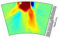
Checkerboard tests show that
alternating low and high velocity anomalies with depth
will be smeared into one continuous LVA when near-vertical
rays are used. This critical test is not performed
by Wolfe et al. (2009) who use vertical prisms instead,
with continuous low-velocity anomalies with depth.
I have prepared a short Powerpoint
tutorial that may be of interest.
4th January, 2010, Don L. Anderson
Resolution tests
It is not generally appreciated, apparently,
that near-vertical teleseismic waves (S, SKS, P. PKP,
ScS, Sdiff) have limited capabilities for determining
absolute velocities and depths of anomalies. Those
studies that use relative arrival times (e.g., Wolfe
et al.,
2009) have no constraints whatsoever on whether
the underlying mantle is slow or fast.
Simple arithmetic shows that vertical
rays traversing a checkerboard test pattern composed
of alternating high and low velocity blocks, with equal
relative velocity perturbations and zero mean, will
end up with a delay, or positive residual. This is
because the rays spend more time in the low velocity
blocks. This prediction is confirmed by elaborate checkerboard
tests of rays emerging at Hawaii (Lei
& Zhao, 2005).
If the test pattern has equal and opposite temperature
perturbations, the predicted slow anomalies are even
more effective because of the non-linear effects of
temperature on seismic velocity. Velocity lowering
is even more extreme if the temperature excursions
lead to melting. The net result is that inversion of
teleseismic arrivals to Hawaii cannot help but find
a low velocity cylinder under Hawaii...even under ideal
checkerboard conditions.
The depth extent of the cylinder
depends on the corrections for shallow structure, the
allowable velocity perturbations, the effects of anisotropy
and smoothing. Wolfe et al. (2009) argue that
shear velocity perturbations in the shallow mantle
cannot exceed 4%, about half what is observed under
Yellowstone, the Rio Grande Rift and the Lau Basin,
and much less than observed across fault and suture
zones, even ancient ones. This assumption dictates
the depth extent of their S-wave anomaly. The depth
extent of the SKS anomaly is based on a homogeneous
lower mantle and an isotopic upper mantle. Even the
relative S-wave variations across the Hawaiian array,
the only source of data, are no more than across the
Canadian Shield.
More generally, in regions of sparse
coverage, such as the Pacific, resolution tests find
only the low velocity patches and the whole underlying
upper and midmantle will appear to be slow (Li
et al.,
2008). Normal mode, surface wave and surface bounce
data are required to actually determine the velocities
in the mantle under the Pacific.
Lei & Zhao (2005) present
a test model with a uniform pattern of high and low
velocity blocks. Near vertical rays (P, PKP, S, SKS)
convert this pattern to a vertical slow cylinder (Lei & Zhao,
2006, p. 438-453).
Contrary to implications in recent
papers, relative teleseismic delay times cannot determine
absolute seismic velocities or temperatures under Hawaii.
They cannot even determine relative velocity perturbations
or depths. The data cannot show, as claimed, “that
the Hawaiian hot spot is the result of an
upwelling high-temperature plume from the lower mantle" (Wolfe
et al.,
2009, abstract).
The apparent plume tilts downward toward the southeast,
in conflict with studies by Montelli
et al. (2004)
(to the W), Lei & Zhao (2005)
(to the S) and Wolbern et al. (2006) (to the
NE). The neglect of the unique upper mantle anisotropy
around Hawaii (Ekstrom & Dziewonski, 1998) creates
an additional delay of 0.8 s in SKS, which Wolfe
et al. (2009) attribute
to the lower mantle portion of their conjectured plume.
Lower mantle structures have been observed to give
SKS delays of 6 s, even when S is normal. Shear
zones extending to 200 km can give delays of 2 s
(RISTRA).
Lei & Zhao (2005) argue
that the LVA anomaly under Hawaii (2000 km across!)
is continuous to the CMB. This is partially because
of their color scale and the orientation of their cross
section. Other color scales and other cross sections
(e.g., Ritsema, 2005) show that the
lower mantle features are disconnected from the upper
mantle ones. Map views show that the feature changes
shape, orientation, intensity, size…with
depth…with the largest change occurring at 600
km, as in Wolfe
et al. (2009).
If it is a continuous feature it widens as it rises
into the low viscosity upper mantle and is therefore
not a buoyant upwelling, nor need it be rising. This
huge feature, if buoyant, should be evident in residual
geoid and topography.
The 650 km discontinuity should be
elevated substantially in a broad region to the NW
of Hawaii but in fact it is no shallower than
it is under ridges or
the S .Pacific, depending on author, and shear
velocities are not particularly low in the transition
zone NW of Hawaii. Wolbern et
al. (2006) argue for
a SW source (and not a SE source) for the Hawaiian
plume, based on elevations of the 650 km discontinuity.
There is also the matter that station
residuals for P and S waves to Hawaii are not particularly
anomalous.
In summary, regardless of what the
mantle under Hawaii looks like, if no mistakes are
made, teleseismic data will image a deep low- (relative
and absolute) velocity cylinder.
5th January, 2010, John R. Evans
Vertical resolution
in teleseismic tomography is (almost) all about
the interaction of ray crossfire with anomaly shape.
This is also true for resolution in general for
all forms of tomography, though additional issues like
strong nonlinearity crop up when turning points and
strongly-coupled parameters are in the model volume).
For issues related to relative times,
perhaps you are thinking of the problem with quasi-horizontal
features such as a possible magma pooling at Yellowstone,
which I think creates a horizontal, mafic lens of very
low velocity near or a bit above Moho. Any such feature
will resolve pretty well at the edges ("well" in
the sense of contrast, not absolute levels or v(x)
shape) and very poorly in the center, eviscerating
that into a diamond shape that is very weak but thick
in the center, about 1.5 times as high as wide in the
crust when using P or S. That central part can be effectively
invisible in the model.
The problem with SKS and PKP (not
S and P to nearly that degree) is that even well into
the upper mantle these rays are very close to vertical–a
few degrees off at best–so that adequate crossfire
is impossible below the depth of good P and S crossfire–the
situation at Hawaii (as Wolfe
et al. (2009) point
out, but then go on to push interpretations beyond
the capabilities of the data). For this reason, the
1500-km deep smear of low is quite clearly an artifact
derived from shallower, more anomalous structures,
or at any rate one cannot demonstrate the contrary,
resolution kernels and checkerboards clearly notwithstanding.
This is a game of the sum of many small numbers in
a noisy, damped system for which numerous approximations
and parameterizations have had to be been made. The
same holds for the deep NW-dipping anomaly at Yellowstone–pure
bunk that no properly experienced tomographer would
give a second glance at.
On the issue of diffractions, yes,
leading diffractions appear in waveforms recorded "down
wind" of
a velocity low. But the (visual, correlative, cross
checked) methods used by a good tomographer are virtually
immune to this problem and readily track the larger
direct wave to perhaps 4-5 anomaly-diameters behind
the anomaly. I have seen (and ignored) such diffractions
in a number of studies.
Unfortunately, most tomographers use
the Van
Decar & Crosson (1990) wide-window numerical-correlation
algorithm to pick and do very little visual cross check
and debugging of the new, giant data sets. Unless a
method that correlates only the largest early peak
or trough is used, this method must subsume significant
systematic errors–the very signals used to compute
receiver functions as well as diffractions. These systematic
errors will map to something in the model and what
will be effectively impossible to identify, though
probably with a tendency to map toward the top or bottom
of the model.
I believe I'm about the 6th person
to practice teleseismic tomography on this planet (7th
for any form of tomography), and almost certainly am
the most experienced of these, with 17 years more or
less continuous work, including numerous numerical
tests of the method. I fear I have become the dreaded
Survey Curmudgeon and am convinced that there still is no-one else out there (except my students!) who
fully understand the perils and pitfalls of the technique
in its full glory–cf. Evans
& Achauer (1993). New techniques (since ACH)
have wowed everyone now practicing into a misplaced
sense of security in trade for some second-order improvements
over ACH (nil improvements over ACH as practiced by
Evans
& Achauer, 1993).
On how anomalous the upper mantle
can get, I'd side with Helmberger for S (perhaps 5%
for P) with the addition of suspected lenses like Yellowstone's.
At Yellowstone, it is clear that 1 - 1.5 s of the
~2 s intra-caldera P delay is due to the upper crustal
anomalies (very strong) and the magma lens (< ~50
km deep) while the upper mantle is consistent with
a partial melt +/- melt channels (likely + in Hawaii
in the deeper seismic zone).
5th January, 2010, Don L. Anderson
The upper mantle can be as much as 5% slow for P
under Hawaii, meaning about 10-15% for S. I
think Jimez is about 8% spread over 200 km. Alpine
fault is reported to be 35% slow for P (high pore pressure?).
Magma/mush can get outrageously slow and, in contrast
to dry porosity, this does not get suppressed by pressure.
What are the chances that there is a 40 km wide, 200
km deep fissure-mush zone under the Hawaiian volcanic
ridge?
If 1 to 1.5 s of delay can be explained by upper crustal
anomalies, as at Yellowstone, this would certainly
explain the S-delays across Hawaii. 6% anisotropy
(Ekstrom & Dziewonski, 1998) can take care of the SKS
part.
Incidentally, do we know the absolute travel times
to Hawaii? Is S slower than to western North America?
5th January, 2010, John R. Evans
Absolute velocities are utterly invisible with relative
residuals. The way that plays out for a thoroughgoing
layer of any velocity is that you cannot see it at
all. But if one has a discontinuous layer like a
lens or the edge of one terrain against another,
the contrast can be determined well across the boundary
but the shape of the anomaly will be very different.
I see no way to get to absolute velocities without
lots of turning points and entire raypaths within the
modeled volume. This is the case for local-event tomography
in which case (x,y,z,t) for events are also in the
mix, along with their z-t tradeoffs. All this leads
to very badly behaved nonlinearity that has led to
numerous garbage results in the literature.
Crossfire and resulting resolution
are determined by the ray density and (hopefully minimal)
isotropy in the five axes of any ray segment: (x,y,z,a,i).
So one wants as many azimuths and
incidence angles as possible and as large an array
aperture and as dense a station spacing as possible,
with smoothness in these things ranging from important
to essential. This figure below, from Evans
& Achauer (1993), illustrates
where one can and cannot expect good resolution.
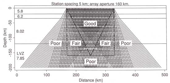
Figure from Evans
& Achauer (1993)
Checkerboard
tests are not useful, regardless of their popularity.
Core phases do have some nonzero
incidence angle. They can
help a little,
but one must have a well-designed array and a well-chosen
set of sources varying broadly in azimuth to recover
anything. The primary efficacy of core phases
is to add another incidence angle in the region with
good mantle-phase crossfire. After that, all one can
hope to say (with limited confidence) is that there
is something additional out along such-and-such a ray
bundle, P(a), S(a), PKP, and SKS. You can have virtually
no idea where along that ray bundle it lies, and smearing
of shallow features makes even this much dicey.
Anisotropy definitely can have such
effects and these would model pretty easily into a
vertical smear below the region of good crossfire.
It is a poorly explored issue.
A 40 km wide, 200 km deep fissure-mush zone under
the volcanic ridge is perfectly plausible but I'd place
my bet on artifact for the deep anomaly.
7th January, 2010, John R. Evans
The results are very interesting in the upper
500 km and the array is well enough designed to support
that pretty well. However, anything deeper is completely
unsupported by the data and the method. Unfortunately,
all that shallow interesting and probably OK part is
color-saturated in the Science paper and thus not available
for interpretation.
It seems the Van Decar & Crosson (1990)
picking method was used and it is not clear if the
result was human-checked. There may well be additional
artifacts from using this picking method incorrectly.
I may have been the first to try stripping off the
signal of shallow structure or otherwise forcing modeling
within a limited depth range (in order to "see
through" strong, shallow anomalies), but I'm not
sure exactly what was done here. I am sure such stripping
in no way informs whether the artifacts are artifacts,
though it might reduce their magnitude. In any case,
the initial model space should not extend much below
500 km since nothing isresolved below this depth
in any meaningful way (one ignores the bottom layer
since that soaks up a lot of the leftover signals that
one cannot model properly).
The array is well-designed to support
tomography in the upper 500 km, as mentioned above,
and a good result can be had from the data. The
data set very likely would also work well to reveal
any CMB-plume guided phases (think optical fiber: Julian
& Evans, in press).
Finding such phases would be strong evidence for a
CMB plume while not finding them in a data set good
enough to see them would be pretty good evidence for
the absence of such structure (but not the slam-dunk
of finding them). It's the only seismic method I know
of that has meaningful potential for finding a weak,
long, skinny, deep anomaly.
7th January, 2010, Don Anderson
The total relative S delays
in the Hawaii experiment are ~2-3 seconds. It is hard
to convert these to absolute delays but absolute P
delays to Hawaii order 1 s are not extreme by global
standards.
However, the paper of Wolbern et al. (2006),
contrived as it is, does show that S wave delays above
410 and between 410 and 650 range up to 3 s,
with no lower mantle involved. These of course depend
on both velocity and discontinuity depths but they
show that maybe there is plenty of variation above
650 or even 400 to explain it all.
7th January, 2010, John R. Evans
Those numbers (P & S) fit reasonably well
for shallow partial melts and melt-filled fractures,
but I must admit to being a little out of date on the
theoretical and lab work on partial melts etc.
9th January, 2010, Alexei Ivanov
Is any chance of getting the
essence of these comments published in the white literature?
9th January, 2010, Gillian R.
Foulger
I would think that a re-processing
of the data would be expected, demonstrating that
the claims of poor resolution are true.
11th January, 2010, John R. Evans
The usefully resolved depth of any teleseismic tomography
study is approximately equal to the array aperture.
The array in question is reasonably well designed for
a study reaching ~500 km beneath the big island but
not deeper – the data cannot return interpretable
results below this depth in the presence of shallow,
strong anomalies, notwithstanding efforts to "strip" shallow
structure, to remove whatever signal can be attributed
to the surface. Stripping can help some, but because
the inversion is damped, some of the shallow signal
will remain in the observations and will be subject
to smearing.
The best-resolved
volume in any ("restricted
array",
i.e., regional) teleseismic tomography is an
inverted cone with its "base" at
the array at the surface and its vertex beneath the
center of the array at a depth about equal to the array
aperture. This is the volume in which one can obtain
mantle phases from numerous azimuths and moderate incidence
angles +/- core phases at near vertical. Even here,
the ratio of vertical to horizontal resolution is roughly
0.5 and inhomogeneity in the ray distribution in 4D
can cause more than the usual artifacts.
In the remainder
of a cylinder beneath the array and of diameter and
depth range equal to the array aperture one has mantle
phases from a narrow range of azimuths plus a core
phase so the resolution is fairly good but with more
radial (here, depth) smearing than within the cone.
At flatter angles outside this cylinder (larger incidence
angles) and below the resolvable depth, the bottom
of the cylinder (~500 km here) where there are only
separated bundles of rays of nearly the same orientation
and there is very little resolution
and terrible smearing – this separation is well illustrated by some of the
supplementary information provided by Wolfe
et al. (2009).
At best one can suggest that there is some remaining
traveltime anomaly somewhere off in those general directions
with no idea where along those separated ray bundles
the anomalies lie (yes, including all the way back
to the surface at the array). Worse, when the features
out there are significantly weaker than the shallow
anomalies (cf. recent Yellowstone and Hawaii work)
one can have absolutely no confidence in those nil-resolved
regions and the presumption must be that those streaks
are entirely artifacts of shallower (including upper
crustal) anomalies of greater strength coupled with
the damping effects of the inversion process (damping
will always push the minimum of the model toward
more but fainter smearing – "shorter" models
– at the expense of a poorer fit to the data). That
is, radial artifacts are a necessary result of shallower
anomalies resolved by any (effectively-)damped inversion
and are taken seriously by no-one well experienced
in the method. Ample evidence of such effects are given
in numerous figures in Evans & Achauer (1993).
To
these problems add the systematic picking errors returned
by the method of Van
Decar & Crosson (1990)
when used with a correlation window wider than
about two seconds beginning at or near the first arrival.
In the presence of such systematic picking errors,
the smearing will tend to worsen; those errors must
find a home in the model – be converted into spurious "anomalies" –
and the easiest (least otherwise constrained) regions
into which to add such spurious signals is in the otherwise
nil-resolved region below and beside the stubby cylinder
described above and shown in the figure.
The issue of
whether smearing can happen with such a data set is
already fully answered: smearing always
will be present in this class of methods and anomalies; the phenomenon
requires no additional demonstration in particulars
because it is a well known, well understood effect.
Indeed, Evans & Achauer (1993) show a
whole series of tests showing the "I on X" smearing
patterns to be expected as the norm and the vertical
elongation of equant anomalies into roughly 2x1 upright
model features.
As we've discussed, these issues do
not preclude the possibility of a weak, deeper feature
– such features are simply un-demonstrated by the present
data and, indeed, cannot be demonstrated with any confidence
at all by that data set. It is a potentially great
data set for looking at the upper 500 km but useless
below that and there should be no other expectation
from such studies.
Finally, checkerboard tests of damped
inversion schema prove only that it's a damped inversion
method – they are useless as tests of resolution,
indeed worse than useless because they badly overstate
whatever resolving power the data have. This is so
because all damped inversion methods prefer to resolve
oscillatory structures, even to the extent that if
given an ill-constrained starting model/data combination
the inversion inevitably will return blocky results,
even in the case of pure noise input to the model.
(Such blockiness is useful as a symptom of the underdamping
of a noisy data set and/or the use of blocks that are
too small – that is, of asking too much of the data.)
The only meaningful resolution tests I know of are
to look at individual resolution kernels (columns of
R or the crudely equivalent one-block or -node synthetic
models using an identical ray set); several one-block
examples should be provided for each of the various
regions outlined in the ray figure from Evans & Achauer (1993),
reproduced above.
Even this exercise is of finite efficacy because of
the issues of parameterization, linearization, and
long sums of tiny numbers, which can have non-obvious
results (which must be assumed present unless otherwise
demonstrated ... how is unclear). Call these one-block
models or kernels the local "impulse
response" of
the data set and inversion method but remember the
long string of simplifying assumptions built into even
these.
29th June, 2010, Don L. Anderson
I
have been waiting for someone better qualified
than myself to comment in Science or Nature on the Wolfe
et al. (2009) Hawaii paper, and and others that
basically use a vertical tomographic (ACH) approach
to mantle structure. The claims in these papers are
compelling to non-seismologists (including journal
editors). Most seismologists
have gone beyond this type of study but they
are still widely quoted, by non-seismologists, and
even referred to as "the highest resolution studies
out there...". I am working on an Appendix to a current
paper and I would appreciate the thoughts of others.
30th June, 2010, Adam M. Dziewonski
Don: It has been known for over 100 years (Herglotz-Wiechert)
that you cannot uniquely determine a velocity profile
if you do not have data for rays that bottom in a certain
range of depths (low velocity zone). What you call "vertical
tomography" is an attempt to circumvent
this law. This is achieved by assuming a starting model
and seeking perturbations to it by imposing additional
conditions of minimum norm or minimum roughness.
The problem with studies such as that
of Wolfe et al. (2009) is that they infer
a structure for which they have only data with a very
limited range of incidence angles at lower (and upper
mantle depths).
This misconception
has been propagated for over 30 years beginning with
the 1977 paper by Aki and others. Using teleseismic
travel times observed at NORSAR they inferred 3-D structure
using rays with a very limited range of incidence angles.
In contrast, Dziewonski et al. (1977) also used teleseismic
travel times but limited their inversion to the lower
mantle, in which it is possible to have all incidence
angles from vertical to horizontal.
Structures obtained
through inversion of data with a limited range of
angles of incidence are highly nonunique, yet the tradition
of such inversions continues with dozens of PASSCAL-type
experiments. An example is the Yellowstone hotspot,
where a slow structure had been claimed at depths exceeding
the aperture of the array.
30th June, 2010, John R. Evans
Adam: I think you too overstate the issue but arrive
at the correct bottom line (with minor exceptions).
The problem here is not ACH tomography and its numerous
(almost exactly equivalent) offspring. The problem
is the newbees to tomography (and folks outside that
specialty), who do not understand the art and limitations
of (restricted array) TT.
It has been known and widely stated from the very
beginning that absolute velocities are utterly unknown
in TT (and by corollaries that Ellsworth, I, and Uli
Achauer established long ago that there are other structures
that can effectively disappear or be misunderstood
more easily than properly understood (I still think
there is a lenticular mafic-silicic "heat exchanger" near
Moho at Yellowstone, for example). The tradeoff in
full-ray tomography at any scale from exploration to
local to global is that the inverse problem becomes
highly nonlinear and very sensitive to starting models
and how cautious the driver is on that jeep track.
So please don't go throwing out baby with bathwater.
TT is a powerful and highly linear, robust (in practice,
if in not theory) method with a great deal to offer
and has made major contributions where no other method
yet dares to go. (Yeah, we'd all love to see full waveform
tomography with all sources and constraints from other
methods, but it ain't here yet. Even then, I guarantee
that it will take 20 years of some curmudgeon like
me hacking away to really understand the beast -- there
is always more than meets the math.)
The problem is not the method but that newbees forget
the art and the geology that are so essential to getting
it right and simply go tunnel visioned on the maths,
checkerboards, and pretty pictures (scaled for convenience
and bias).
Every geophysical method has limitations, which must
be well understood or it is useful in, garbage out.
The Evans & Achauer (1993) chapter 13 in Iyer's great,
pragmatic book on the art of tomography was an attempt
to established a Perils and Pitfalls for TT, as was
done famously and long ago for reflection seismology
(e.g., no, the Earth actually is not composed largely
of hyperbole ... only some papers!).
This subject really
is worthy of a new paper of its own in a lead journal,
a paper redolent in crisp, definitive statements to
clarify some things that seem to have been forgotten
in recent years.
2nd July, 2010, Jeannot Trampert
Don: I am not sure mere comments are going to change
the perception of the subject. There seem to be two
camps, the people who understand the limits of the techniques
and those who project wishful thinking into the results
obtained by the same techniques. There have been many
comments and replies in the published literature but
the debate has remained polarized.
The problem is of course
that we do (could) not estimate uncertainties related
to tomographic results. If people knew that anomalies
carry uncertainties of the order of 1% (for example),
they would refrain from interpreting anomalies of 0.5%.
Very often resolution and uncertainty are confused.
While there is a relation, they are not the same. You
can infer a broad average very accurately, while a
local property often carries a large uncertainty.
Checkerboard
tests are very dangerous, because they are used to
convince people that there is resolution while the
mathematics tell you the opposite.
Rather than another
comment, I think a tomographic study is needed with
a complete uncertainty analysis. We are working on
this here in Utrecht, but the calculations are long.
2nd July, 2010, John R. Evans
I agree with Jeannot. R is not
C and both subsume a lot of physics
and maths assumptions. I hope Jeannot and his colleagues
have good success in a better evaluation.
See Can tomography
detect plumes? for continuation of this discussion.
References
-
Ekström, G., and A. M.
Dziewonski (1998), The unique anisotropy of the
Pacific upper mantle, Nature, 394,
168-172.
-
Evans, J. R., and U. Achauer, 1993, Teleseismic
velocity tomography using the ACH method: theory
and application to continental-scale studies, in
Seismic Tomography: Theory and
Applications, edited
by H. M. Iyer and K. Hirahara, pp. 319-360, Chapman
and Hall, London.
-
Julian, B. R., and J. R. Evans (2009), On possible
plume-guided seismic waves, Bull.
seismol. Soc. Am.,
in press.
-
Katzman, R., L. Zhao, and T.H.
Jordan, 1988, High-resolution, two-dimensional
vertical tomography of the central Pacific mantle
using ScS reverberations and frequency-dependent
travel times, J. geophys. Res., 103,
17,933-17,971.
-
-
Li,
C., van der Hilst, R.D., Engdahl, E.R., and Burdick,
S., 2008, A new global model for P-wavespeed
variations in Earth's mantle, Geochemistry,
Geophysics, Geosystems, 9,
Q05018, doi:10.1029/2007GC001806
-
Montelli,
R., Nolet, G., Dahlen, F.A., Masters, G., Engdahl,
E.R. & Hung, S.-H., 2004,. Finite frequency
tomography reveals a variety of plumes in the
mantle, Science, 303, 338–343.
-
-
Ritsema, J. (2005), Global seismic
maps, in Plates, Plumes & Paradigms,
edited by G. R. Foulger, J.H. Natland, D.C. Presnall
and D.L. Anderson, pp. 11-18, Geological Society
of America.
-
-
Wolbern, I., A.W.B. Jacob, T.A.
Blake, R. Kind, X. Li, X. Yuan, F. Duennebier & M.
Weber, 2006, Deep origin
of the Hawaiian tilted plume conduit derived from
receiver functions, Geophys.
J. Int., 166,
767–781.
-
last updated 2nd July, 2010 |