 |
The probability of mantle plumes in global tomographic models |
Augustin Marignier1,2, Ana M.G. Ferreira2,3 & Thomas Kitching1
1Mullard Space Science Laboratory, University College London, London, UK; augustin.marignier.14@ucl.ac.uk ; t.kitching@ucl.ac.uk
2Department of Earth Sciences, University College London, London, UK, 3CERIS; a.ferreira@ucl.ac.uk
3Instituto Superior Técnico, Universidade de Lisboa, Lisboa, Portugal
This webpage is a summary of Marignier, A., A. M. G. Ferreira, and T. Kitching (2020), The Probability of Mantle Plumes in Global Tomographic Models, Geochemistry, Geophysics, Geosystems, 21, e2020GC009276.
Introduction
Seismic tomographic models are derived from our most direct observations of the deep Earth and are thus our best chance to see plumes and how far down they extend. The issue is that tomographic models tend to disagree, particularly when it comes to smaller scale structures. These differences are likely due to the different seismic datasets, inversion schemes and parameterisations, and forward modelling schemes used by different studies. Furthermore, a general loss of resolution at greater depths makes it very difficult to see the depth extent of possible plumes. With no reported uncertainties, interpreting as mantle plumes features seen visually in tomographic models becomes quite subjective. The aim of our study is to objectively quantify some measure of probability that a seismic anomaly may resemble a mantle plume and use this to assess the level of agreement between a set of seven recent global shear wave velocity models.
Method
To define some measure of probability without any reported uncertainties, we assumed that each tomographic model was a sample of a statistical distribution, and that the difference between samples from said distribution is high-frequency noise. We simulate this distribution by simulating the high frequency structures of the model. This is done by taking the spherical wavelet transform of the model. The wavelet transform is similar to the Fourier transform in that it returns the frequency content of a signal, but the wavelet transform also returns where in space the different frequencies arise. So, by taking the spherical wavelet transform of a tomographic model, we can replace the highest frequency information with some different, but spectrally similar, high frequency noise. Repeating this means that for each tomographic model we generate 500 slightly different versions, i.e. samples from a statistical distribution. We then analyse this distribution and define a probability that plumes stand out from the noise that we have simulated.
We define our plume probability using the very simple assumption that a plume comprises a vertically continuous low-shear-velocity anomaly according to a signal-to-noise ratio test statistic. We allow for possible plume tilt of 10° by tiling the Earth into 8°´8° tiles. However, with the aim of being as general and objective as possible we do not account for any more complicated structures that occur in geodynamic simulations or are reported from visual examination of tomographic models. This way we can define a plume probability for every point on the Earth, and as such possibly detect a previously unreported plume-like features. Had we accounted for different complexities such a definition would not be possible. Full details of the statistical calculations can be found in our paper (Marignier et al., 2020)
Results
For each tomographic model, a global map of plume probability is produced. We find that for all the models, probabilities greater than 50% are concentrated beneath much of the African continent and the Pacific Ocean. This suggests some correlation with the Large Low Shear Velocity Provinces (LLSVPs), thermochemical piles of material at the bottom of the mantle which are suspected to have some link to the origin of deep plumes.
Figure 1 shows a vote map where each tomographic model gives a vote to the tiles where it has assigned a plume probability greater than 94%. The standout regions where most of the models agree on high plume probability are East Africa and the central Pacific hotspots, as well as Iceland and Hawaii. We also see some agreement near the Marion, Kerguelen and Crozet hotspots, and near the Amsterdam-St Paul hotspot further east. In these areas we find clusters of single votes, suggesting that our method has detected features in the models, but a paucity of seismic stations makes precisely locating them more challenging. The Amsterdam-St Paul hotspot has only been associated with a deep plume in one other tomographic study (Zhao, 2007), whereas geochronology and composition studies (e.g., Janin et al,. 2012) have concluded that there must be a deep plume here. This is evidence that our method and potentially future similar numerical studies have the ability to detect features that can be missed upon visual inspection of tomographic models.
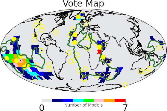
Figure 1: Vote map where the seven tomographic models vote for every tile in which they have a plume probability greater than 94%. Yellow dots are the “primary plumes” of French & Romanowicz (2015), yellow circles are the other hotspots of Courtillot et al. (2003). Green lines show the outlines of the LLSVPs according to Cottaar & Lekic (2016).
We analysed in further detail a set of 50 known hotspots and classified them into four categories based on the distribution of probabilities assigned by the seven models (Figure 2). The four categories describe where deep plumes are “highly likely”, “likely”, “unclear” or “unlikely”. Our “highly likely” plumes include Macdonald, Tahiti, East Africa and Hawaii, whereas our “unlikely” plumes include Yellowstone and Juan de Fuca. Encouragingly, our classification largely agrees with a ranking of deep plumes at hotspots from a previous study (Boschi et al., 2007) that made comparisons between some older tomographic models and geodynamic simulations. This shows that despite our very general definition of a plume, we were able to detect plumes that may have much more complicated structures. Furthermore, a key difference with that study is that we have classified the Marquesas and Pitcairn hotspots as much more likely. We see a very good agreement between the more recent tomographic models used in our study, suggesting that tomography is progressing and improving the resolution of smaller scale features. Finally, our “highly likely” and “likely” plumes can be found around the edges of the LLSVPs and the “unlikely” plumes are found away from them. This supports theories that plumes are created when the convecting mantle or subducted slabs run into these large thermochemical piles (e.g., Steinberger & Torsvik, 2012; Ballmer et al., 2016).
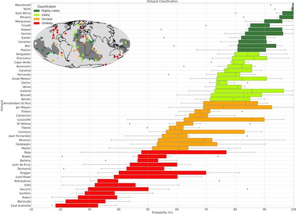
Figure 2. Boxplots of probabilities across seismic tomography models of the hotspots of Courtillot et al. (2003), in addition to Amsterdam-St Paul and East Africa but without Meteor. Coloured boxes show the interquartile range (IQR) of probabilities, with the vertical line inside the box representing the median probability. Colours are based on our plume classification, which is determined by the lower quartile. The error bars extend to the lowest probability within 1.5 IQR beneath the lower quartile (left end of boxes) and to the highest probability within 1.5 IQR above the upper quartile (right end of boxes). Any probabilities beyond 1.5 IQR from either quartile are considered outliers and shown as black diamonds. Inset map shows hotspot locations with colours corresponding to the plume classification. Dark patches are the LLSVPs of Cottaar & Lekic (2016). Click here or on Figure for enlargement.
Summary
In this study, we have argued that interpreting tomographic models visually without uncertainties can be misleading and cause features to be missed. We have presented an alternative numerical method to objectively assess the presence of plumes in individual models and identify the similarities and differences. Detecting a plume that seems to have previously been missed indicates that this sort of numerical assessment is an important way forward. Furthermore, we have presented a classification of the most likely vertically continuous low velocity anomalies which should contribute further to the ongoing plume debate.
References
-
Ballmer, M. D., Schumacher, L., Lekic, V., Thomas, C., & Ito, G. (2016). Compositional layering within the large low shear-wave velocity provinces in the lower mantle. Geochemistry, Geophysics, Geosystems, 17, 5056–5077. https://doi.org/10.1002/2016GC006605
-
Boschi, L., Becker, T.W., & Steinberger, B. (2007). Mantle plumes: Dynamic models and seismic images. Geochemistry, Geophysics, Geosystems, 8, Q10006. https://doi.org/10.1029/2007GC001733
-
Cottaar, S., & Lekic, V. (2016). Morphology of seismically slow lower-mantle structures. Geophysical Journal International, 207(2), 1122–1136. https://doi.org/10.1093/gji/ggw324
-
-
-
Janin, M., Hémond, C.,Maia, M., Nonnotte, P., Ponzevera, E., & Johnson, K. T. M. (2012). The Amsterdam-St. Paul Plateau: A complex hot spot/DUPAL-flavored MORB interaction. Geochemistry, Geophysics, Geosystems, 13, Q09016. https://doi.org/10.1029/2012GC004165
-
-
Zhao, D. (2007). Seismic images under 60 hotspots: Search for mantle plumes. Gondwana Research, 12(4), 335–355.
last updated 2nd November, 2020 |
