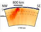
Structure under
Hawaii, from Li et al., Geochem. Geophys. Geosyst., 9,
Q05018, 2008. |
Can
tomography detect plumes?
Discussion |
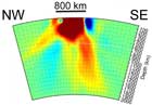
Structure
under Hawaii, from Wolfe et al.,
Science, 326, 1388-1390,
2009. |
See also Hawaii Plume Discussion
29th June, 2010,
Don L. Anderson
I
have been waiting for someone better qualified
than myself to comment in Science or Nature on the Wolfe
et al. (2009) Hawaii paper, and others that
basically use a vertical tomographic (ACH) approach
to mantle structure. The claims in these papers are
compelling to non-seismologists (including journal
editors). Most seismologists
have gone beyond the recent Science and Nature papers
but they are still widely quoted, by non-seismologists,
and even referred to as "the
highest resolution studies out there...".
30th June, 2010, Adam M. Dziewonski
Don: It has been known for over 100 years (Herglotz-Wiechert)
that you cannot uniquely determine a velocity profile
if you do not have data for rays that bottom in a certain
range of depths (low velocity zone). What you call "vertical
tomography" is an attempt to circumvent
this law. This is achieved by assuming a starting model
and seeking perturbations to it by imposing additional
conditions of minimum norm or minimum roughness.
The problem with studies such as that
of Wolfe et al. (2009) is that they infer
a structure for which they have only data with a very
limited range of incidence angles at lower (and upper
mantle depths).
This misconception
has been propagated for over 30 years beginning with
the 1977 paper by Aki and others. Using teleseismic
travel times observed at NORSAR they inferred 3-D structure
using rays with a very limited range of incidence angles.
In contrast, Dziewonski et al. (1977) also used teleseismic
travel times but limited their inversion to the lower
mantle, in which it is possible to have all incidence
angles from vertical to horizontal.
Structures obtained
through inversion of data with a limited range of
angles of incidence are highly nonunique, yet the tradition
of such inversions continues with dozens of PASSCAL-type
experiments. An example is the Yellowstone hotspot,
where a slow structure had been claimed at depths exceeding
the aperture of the array.
30th June, 2010, John R. Evans
Adam: I think you too overstate the issue but arrive
at the correct bottom line (with minor exceptions).
The problem here is not ACH tomography and its numerous
(almost exactly equivalent) offspring. The problem
is the newbees to tomography (and folks outside that
specialty), who do not understand the art and limitations
of (restricted array) TT.
It has been known and widely stated from the very
beginning that absolute velocities are utterly unknown
in TT (and by corollaries that Ellsworth, I, and Uli
Achauer established long ago that there are other structures
that can effectively disappear or be misunderstood
more easily than properly understood (I still think
there is a lenticular mafic-silicic "heat exchanger" near
Moho at Yellowstone, for example). The tradeoff in
full-ray tomography at any scale from exploration to
local to global is that the inverse problem becomes
highly nonlinear and very sensitive to starting models
and how cautious the driver is on that jeep track.
So please don't go throwing out baby with bathwater.
TT is a powerful and highly linear, robust (in practice,
if in not theory) method with a great deal to offer
and has made major contributions where no other method
yet dares to go. (Yeah, we'd all love to see full waveform
tomography with all sources and constraints from other
methods, but it ain't here yet. Even then, I guarantee
that it will take 20 years of some curmudgeon like
me hacking away to really understand the beast -- there
is always more than meets the math.)
The problem is not the method but that newbees forget
the art and the geology that are so essential to getting
it right and simply go tunnel visioned on the maths,
checkerboards, and pretty pictures (scaled for convenience
and bias).
Every geophysical method has limitations, which must
be well understood or it is useful in, garbage out.
The Evans & Achauer (1993) chapter 13 in Iyer's great,
pragmatic book on the art of tomography was an attempt
to established a Perils and Pitfalls for TT, as was
done famously and long ago for reflection seismology
(e.g., no, the Earth actually is not composed largely
of hyperbole ... only some papers!).
This subject really
is worthy of a new paper of its own in a lead journal,
a paper redolent in crisp, definitive statements to
clarify some things that seem to have been forgotten
in recent years.
2nd July, 2010, Jeannot Trampert
Don: I am not sure mere comments are going to change
the perception of the subject. There seem to be two
camps, the people who understand the limits of the techniques
and those who project wishful thinking into the results
obtained by the same techniques. There have been many
comments and replies in the published literature but
the debate has remained polarized.
The problem is of course
that we do (could) not estimate uncertainties related
to tomographic results. If people knew that anomalies
carry uncertainties of the order of 1% (for example),
they would refrain from interpreting anomalies of 0.5%.
Very often resolution and uncertainty are confused.
While there is a relation, they are not the same. You
can infer a broad average very accurately, while a
local property often carries a large uncertainty.
Checkerboard
tests are very dangerous, because they are used to
convince people that there is resolution while the
mathematics tell you the opposite.
Rather than another
comment, I think a tomographic study is needed with
a complete uncertainty analysis. We are working on
this here in Utrecht, but the calculations are long.
2nd July, 2010, John R. Evans
I agree with Jeannot. R is not
C and both subsume a lot of physics
and maths assumptions. I hope Jeannot and his colleagues
have good success in a better evaluation.
6th July, 2010, Don L. Anderson
All this talk about resolution is nice but beside the
point for this issue. It seems to be overlooked
that the recent Science paper, and earlier ones
in Nature, use only relative delay times over
the small area investigated. Half of the arrivals are
guaranteed to be later than the other half but it needs
to be shown that these are slow in an absolute, global
or regional sense. This has nothing
to do with which approximation is used or what the
resolution is. Confusing relative times with absolute
times is about as fundamental an error as you can make.
If the shallow mantle is as heterogeneous
and anisotropic as workers such as Ekstrom and Dziewonski
say then one can show that the signals recorded by
the Hawaiian array are created above 220 km depth.
Furthermore, the tests by West
et al. (2004) show that
artifacts like those apparent in the results of Wolfe
et al. (2009) are created
by known shallow structures unless surface waves (and
regional seismic phases) are used along with vertical
body waves. Even the authors of the Wolfe
et al. (2009) paper admit
that complex shallow structures (of the very type imaged
by surface waves and receiver functions)
might (will, actually) explain the results. Montelli
and colleagues acknowledge that little is known about
structure above ~300 km but consider this unimportant.
If you can't constrain the shallow mantle you cannot
talk about the deep mantle (for these kinds of measurements).
This is a fundamental.
6th July, 2010, Gillian R. Foulger
While I agree with Don, I
have to disagree on what is the "Occam's razor" approach
to debunking the results of Wolfe
et al.
(2009). Personally I think that it is surely more persuasive
to point out that the experiment fundamentally
cannot resolve a feature where they say one is, rather
than arguing that there are geological complications
(structure, anisotropy etc.) at shallow depth under
Hawaii.
The latter approach will sound to
most people like suggesting an ad hoc model
that is not specifically supported, to explain away
a plume-like structure which is similar to what many
people expect to see. Yes, I know that there is evidence
for anisotropy and shallow structure under Hawaii,
but has anyone published a specific model that could
be subtracted from the data of Wolfe
et al. (2009)
to make the "plume" vanish? And if so, why don't we
need to appeal to such structures to make an Icelandic
lower-mantle plume disappear, or a Yellowstone one?
This will sound to most people like:
Iceland = no LM plume seen
Yellowstone = no LM plume seen
Hawaii = LM plume IS seen, but we explain it away as
anisotropy & shallow structure.
People simply won't find that convincing.
Furthermore, this "plume" could be structure
anywhere along the ray bundle – in the Chile trench,
near the CMB etc. I don't see why it has to be shallow,
or anisotropy. I think we cannot say where along the
ray paths from the hypocenters somewhere in the circum-Pacific
trench system to the surface stations at Hawaii, is
the source of the tiny, much-smaller-than-the-corrections-and-the-errors "plume
signal".
9th
July, 2010, John R. Evans
I agree that sticking to the fundamentals
is the best approach. Teleseismic Tomography (TT) simply
CANNOT resolve location (at most it can tell direction)
below the depth of good ray crossfire (about the array
aperture). In addition to features actually present
ANYWHERE below this array-aperture depth being candidates
for the deeper features in models, note that TT WILL
smear some of any unmodeled shallow perturbations not
removed to those depths because it has no data to counter
that solution and it shortens the model (in a damped
inversion, it is "easier" [lower
mismatch+length error metric] to split the shallow
stuff between shallow and deepest than it is to put
it all shallow, where it belongs).
The zealots will counter that they have removed ALL
shallow structure by "crustal and upper-mantle
stripping" and I can't argue against that very
well without high-quality test models. In fact, I've
made similar claims, though only for the regions WITH
good ray crossfire where the inversion finds it harder
to dump the leftovers.
Doing test models correctly requires full synthetics
of P and S broadband waveforms (up to 2 or 3 Hz) received
above a set of features present only in the crust and
upper mantle (no CMB plume) and picking the arrivals,
debugging the data, and inverting for structure as
per normal.
The picking and debugging should be
done two ways – the lazy, wrong way that is used now
routinely (which subsumes systematic errors from the
receiver function into the residuals) and the right
way, by an experienced human in the painstaking way
it was done for the first 15 years or so. Clearly that's
a lot of work. Also, someone needs to step up for the
synthetics (and instrument transfer functions) and
someone needs to do other types of inversions with
more sophisticated maths.
Note specifically that simple ray
tracing or "ray
front (potential) tracing" are not sufficient
and will not reproduce a true field experiment in the
way we need to nail this. (I think we might easily
get away with using one input waveform to the bottom
of the crustal/upper-mantle anomalous zone and do the
full PDF work only above that depth. That is, assume
perfectly one-dimensional lower crust, core, and source-zone
velocity model. We have not talked about wavefront
healing which would make this a good approximation
even in the presence of modest perturbations in these
places.
Other matters, like anisotropy, would simply confuse
the matter and may not be relevant in any case if one
is simply reading (with steep rays) a vertical alignment
of olivine etc. in response to flow in a hypothetical
plume. Such a feature would look almost exactly like
a simple low or high and any distinction would be second
order or less (one of the reasons that attempts to
account for anisotropy have been pretty weak and not
repeated).
6th July, 2010, Don L. Anderson
The
ban of my life! Anisotropy is not a small effect nor
one that can be corrected out (I wrote a book about
that; Anderson, 1989). In the Pacific the
anisotropy reaches 8% and the drop of Vs into
the low-velocity anisotropic layer is also 8%. Vertical
shear waves are 8% slower than near horizontal SH waves.
Intermediate angle SV waves
can be even slower. Simple arithmetic shows that S
and SKS waves can vary by ~1-2 seconds through
this kind of layer and another second or two can be
added with the kinds of variations in lid thicknesses
that are measured.
Crustal, bathymetry and elevation are comparable.
Heterogeneity below ~200 km then becomes a small perturbation,
not the first order effect.
If one inverts
for anisotropy first, and then for residual
heterogeneity, rather than the reverse, one
becomes a believer! As Dziewonski & I showed many
years ago, if you have a lot of data and are allowed
to fit 12 parameters (degrees of freedom), you get
a much simpler model (structurally) and a better fit,
if you use some of the parameters for anisotropy instead
of a lot of isotropic layers (e.g., as Laske does for
Hawaii).
Pacific anisotropy appears to require
a laminated stack rather than oriented olivine crystals.
Even with no lateral heterogeneity at all (a flat anisotropic
layer) you can do a pretty good job at fitting the
data of Wolfe et al. (2009). If the laminations
tilt to the NW, as predicted, e.g., by Kohlstedt for
melt-rich shear zones, then SKS is explained as well.
Then, you can fiddle with heterogeneity to fit the
rest of the residuals. This seems backwards if you
grew up in an isotropic world.
I suspect that since anisotropy is such a big effect
that if you do the usual of trying to find heterogeneity
first you will have a funny model and then if you try
to fit the residual with anisotropy you might conclude
that "attempts to account for anisotropy [are]
pretty weak"!
9th July, 2010, John R. Evans
I understand that, Don, though thank you for some
new details.
I was simply trying to say: "Imagine
a vertical plug in which the anisotropy is in one direction
while it is some other but monotonous direction in
all surrounding areas and further that is the ONLY
difference between those regions. Because most of the
rays in TT are quasi-vertical, that is still a binary
model – the plug will look different from everything
else around it whether that is (correctly) explained
as anisotropy or (incorrectly) by an isotropic anomaly." You
cannot tell the difference via TT at any meaningful
level of certainty. To see anisotropy as clearly different
from an isotropic anomaly, one must have a broader
range of incidence angles.
8% is comparable to other (shallow) anomaly magnitudes
and bigger than lower-mantle and most upper-mantle
anomalies, so it may well be anisotropy, we simply
can't distinguish.
So "second order" is not
the right term, rather "effectively indistinguishable
by TT".
Where inversions for both isotropic anomalies and anisotropy
have been tried (and you relate an example) the difference
in model fit as a function of causality has not been
resounding. Your Ekstrom & Dziewonski experiments
of reversing the order or adding innumerable parameters
to the fit both confirm my point – many anomalies
can be explained in many ways and the problem is in
distinguishing the various effects in the specific
case of TT. Inter-parameter R and C are very weak with
a typical TT data set. Something will be measured and
modeled but we know not which among the many candidate
causes to blame for it.
In contrast, the negative effects
of the necessarily limited ray set in TT outside the
well-sampled volume are as strong as the objects being
(mis)interpreted – one need go no further than that
to demonstrate the hypothesis – that the various "plume" results
are unsupported by the data cited. I've measured anisotropy
by splitting and know well that it is real – that's
just not the point! KISS to penetrate the doubting
reader's paradigm.
References
-
Anderson, Don L., Theory
of the Earth, Blackwell Scientific Publications,
Boston, 366 pp., 1989.
-
West, M., W. Gao, and S. Grand,
A simple approach to the joint inversion of seismic
body and surface waves applied to the southwest
U.S., Geophys. Res. Lett., 31,
L15615, doi:10.1029/2004GL020373, 2004.
-
last updated 12th July, 2010 |