 |
Is
there convincing tomographic evidence for
whole mantle convection? |
 |
Don
L. Anderson
Seismological Laboratory, California Institute
of Technology, Pasadena, CA 91125
dla@gps.caltech.edu
 Click here to
download a PowerPoint presentation illustrating
this webpage Click here to
download a PowerPoint presentation illustrating
this webpage
Abstract
The approach of visual inspection
of selected tomographic cross-sections, coupled
with the assumption that tomography is simply a
mantle thermometer (red = hot, blue = cold), has
great potential for misleading Earth scientists
who are not seismologists, and even those who are,
but are unfamiliar with the shortcomings of the
particular experiment at issue. Geochemical and
geodynamic interpretations that involve large-scale
mass transfer through the entire thickness of the
mantle are often based on simplistic and indefensible
interpretations of a few brightly colored images
that may have been specially selected to make the
strongest case possible in support of plumes. Seismic
experiments that give superior resolution in particular
areas, i.e., high-frequency, high-resolution studies,
reveal a much more complex mantle than tomography
does–a mantle that is not well explained
by simplistic, conventional models.
The controversy
Allegre (1997) states
that it is increasingly accepted that the Earth’s
mantle has a two-layer structure. This was based
on the standard geochemical two-reservoir, two-layer
assumption. Kamber & Collerson (1999)
claim that growing geophysical and geochemical
evidence continues to support the original “standard” two-layer
model. This is based on the assumption that the
upper mantle is homogenized by vigorous mantle
convection and that if MORB is derived from the
upper mantle, nothing else can be.
At the same time, van der
Hilst et al. (1997 and elsewhere) state
the view, which they describe as a consensus,
that slabs of subducted lithosphere sink deep
into the lower mantle. This contradicts the two-layer
model. It is based on the visual impressions
of a few dramatic color cross-sections and the
assumption that “blue” (i.e., high
seismic velocity) unambiguously represents cold,
sinking, dense slabs. The implication is that
present-day mantle convection is dominated by
whole-mantle flow. Whole-mantle circulation schemes
have subsequently become increasingly complex
(e.g., Meyzen et al., 2007; Bercovici & Karato,
2003).
Tomography
can give an imcomplete or misleading picture
Global tomography is a powerful
but imperfect tool. The whole-mantle convection
interpretation of tomography, although widely held,
particularly in the isotope geochemistry and geodynamic
communities, is nevertheless not a consensus view
of seismologists. Travel-time tomography, used
alone, is particularly limited:
- Seismic ray coverage in the Earth is sparse
and spotty. Many regions are devoid of rays.
This lack of data cannot be remedied by using
improved inversion theories. Any experiment,
including seismic tomography, must deal with
the limitations dictated by the distribution
and quality of the available data, sampling
theory, and trade-offs between diverse structures
within the Earth (Spakman & Nolet,
1988).
It is likely that the Earth possesses a substantial
component in the null-space of any mix of data
(e.g., Shapiro & Ritzwoller, 2004).
This is also true for isotope data and box
models. Methods are available to control the
over-interpretation of sparse data, but these
guarantee neither physical acceptability of
the resulting model nor a model that resembles
the real Earth. Simply put, if a region is
not sampled by seismic waves, its structure
cannot be retrieved by tomography or any other
seismic experiment. This remains true despite
published maps and cross sections that include
these regions along with adjacent, well-sampled
regions.
- The visual appearance of displayed results
can be radically changed by adjusting the color
scheme (Figures 1-3) or reference model, smoothing,
cropping, or carefully selecting cross-sections.
The resulting images may be convincing but
are in truth misleading (Spakman et al., 1989).
Images that were not selected for publication
may give a completely different impression.
- The results depend crucially on the ray geometry,
which is constrained by the geometry of the
earthquakes and seismic stations (see Vasco
et al., 1994 for maps of the coverage)
and, to a lesser extent, by the details of
the mathematical techniques employed (Spakman & Nolet,
1988; Spakman et al., 1989; Shapiro & Ritzwoller,
2004).
- Presently existing algorithms and inversion
methods cannot correct completely for various
problems such as anisotropy, the finite frequency
of the seismic waves used and earthquake source
complexities.
- Global tomographic models have poor resolution.
Other studies involving, for example, high-frequency
reflections, scattering, and coda waves, reveal
a more complex picture of the mantle than is
available from tomographic studies that use
long-period waves and large-scale smoothing.
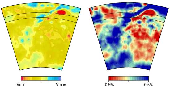
Figure 1. A slab on command!
Line of section traverses Japan (from Ricard
et al., 2005).
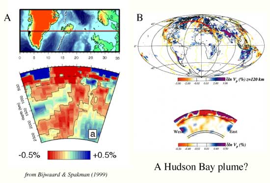
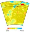
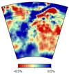
Figure 2. A plume on command.
(A) from Bijwaard & Spakman (1999). Colour
scale saturates at ±0.5% of the anomaly,
which is only a tenth of the strengh of the
upper mantle low-velocity anomaly. (B) same
model is replotted with a colour scale that
saturates only at the strongest upper-mantle
anomalies, and a longer line of section, which
reveals a similar, even more plume-like body,
beneath Hudson Bay.

Figure 3. Cross sections
through Japan showing shallow-bottoming slabs.
Other authors have used a different color scheme
but similar seismic models to “prove” deep
slab penetration (from Fukao et al., 2001).
Color 2D cross-sections are particularly unreliable
for giving a correct impression of the results
of a tomographic study. Although vivid and impressive
to nonspecialists, they are not the overwhelming,
compelling and convincing evidence that they
are commonly presented as being. A few cross
sections cannot adequately express the information
content of a typical 3D tomographic study. A
filtered, smoothed, essentially three-color cross-section
has two orders of magnitude less information
than the original model, which in turn utilizes
only about 1% of the information content of the
seismic waves used (i.e., their arrival times
at stations). In view of this it is astonishing
that sweeping conclusions have been drawn based
on visual inspection of single selected slices
through models.
Seismic
velocity is not a
thermometer
Seismic velocity depends on:
- Phase (i.e., the presence or absence of
partial melt),
- Composition (lithology, mineralogy and
chemistry), and
- Temperature.
There is a fundamental ambiguity problem in
the interpretation of seismic velocities, including
tomographic images, because the effects of
these three factors are not easily separated
out. Of the three, the presence of partial
melt has the strongest effect on seismic velocities
and temperature the weakest.
Nevertheless, tomographic images
are often interpreted assuming that a simple
velocity–density–temperature correlation
exists. High velocity (blue) is generally attributed
to cold, dense, sinking material, and low velocity
(red) as hot, low-density, rising material (Figures
4 & 5). This is unsafe.
Figure 4. The large, red,
2000-km-wide feature extends from the southern
hemisphere under the Shona and Bouvet volcanic
regions up to the Afar region at the surface,
some 7000 km distant. It has been assumed to
be a continuous hot feature that penetrates
the whole mantle, and dubbed a
"superplume" (from Ritsema,
2005).
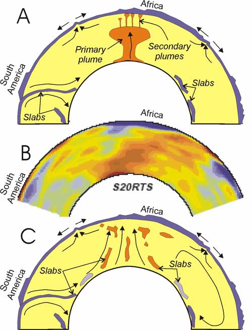
Figure 5. The red tomographic
feature under Africa has been interpreted as
a hot rising plume but it could be a cold iron-rich
sinker, or be neutrally buoyant. A different
color saturation scheme could make the region
under South America appear to be an enormous
blue slab. (from Ivanov,
2005).
High-velocity regions are not
necessarily cold, dense sinkers. Residuum left
after melt extraction, and cratonic roots are
examples of high-velocity material that has low
density and is buoyant. Conversely, eclogite
at ambient mantle temperatures can have low velocities
and a range of densities. The global low-velocity
zone beneath the “mantle lid” has
velocities up to ~20% low compared with the IASP91
standard global seismic velocity model. This
cannot be explained solely by temperature; partial
melt is required (Tan & Helmberger,
2007). The African and south Pacific “superplumes” are
vast, low-velocity bodies in the lower mantle
whose low velocities have been shown to result
from anomalously high density and not to high
temperature (Trampert et al., 2004)
In a peridotite mantle, topography
on the transition zone boundaries may be used
as a proxy for temperature. High-temperature
regions are predicted have thin transition zones.
However, the thickness of the transition zone
shows no correlation with low-seismic-velocity
regions in the lower mantle, with the “superplumes”,
or with upper mantle tectonics. The only correlations
observed are that oceans have relatively thin
transition zones and slab-rich subduction-zone
regions have relatively thick transition zones
(e.g., Deuss,
2007; see also transition
zone pages).
Interpretations
Recent papers defend or present
modifications to the standard one- and two-layer
models of geodynamics and geochemistry (e.g.,
van der Hilst et al., 1997; Kellogg & Wasserburg,
1990; Kellogg et al., 1999), without
changing the basic assumptions of a well-stirred
homogeneous upper mantle, an accessible lower
mantle and a correlation between isotopes and
seismic models (e.g., Helffrich & Wood,
2001; DePaolo & Manga,
2003; van der Hilst, 2004; Meyzen
et al., 2007; Bercovici & Karato,
2003). These represent one particular train of
thought about the accessibilty of the lower mantle
to slabs and surface volcanoes. The non-uniqueness
of tomographic and geochemical models, and compositional
and dynamic interpretations of them, are intrinsic
limitations but are seldom addressed. However,
the non-uniqueness is obvious when one looks
at the large number of published models that
are based on essentially the same data.
Quantitative
seismology vs visual tomography
In qualitative tomography the
reader depends on the visual impression created
by the designer of the published image. Tomographic
cross-sections that have been interpreted as
evidence for deep slab penetration can also be
plotted with different color scales (e.g.,
Ricard et al., 2005) to suggest stagnant
slabs in the upper mantle (Fukao et al., 2001).
The visual impressions given by cross-sections
depend heavily on the orientation and the vertical
and horizontal cropping. Artifacts such as streaking,
bleeding and smearing, the results of sparse
ray coverage, smoothing and unmodeled anisotropy,
are inevitable and may not be obvious if not
pointed out by the authors. A Google Image search
on mantle tomography slabs or slabs
tomography will bring up many images that
could be used to argue in a number of different
ways.
Cartoons should be viewed with
particular skepticism. They are often presented
in order to illustrate a model that is not shown
in any one data set, even using carefully chosen,
cropped and colored cross sections. For example,
when color schemes are chosen to emphasise continuous
red features, blue featues often disappear (Figure
6). Thus, to illustrate conceptual models involving
both upwelling plumes and downgoing slabs, cartoons
may be the only resort (e.g., Figure
5).
Figure 6. When the color
scheme, reference model and cross-sections
are chosen to emphasize continuous red features,
one usually does not see the "whole-mantle
slabs", and vice versa. For this reason,
cartoon interpretations are drawn (the "having
your cake and eating it" approach, e.g.,
Figure 5). This image could have been plotted
differently to make it appear as though there
is a whole mantle slab is under South America
(from Ritsema,
2005).
Quantitative analysis of
tomographic results involves the calculation
of correlations and spectra and quantitative
hypothesis testing. Analyses based on the correlations
between density, shear velocity, and compressional
velocity, for example, are much more powerful
than merely glancing uncritically at a single
cross-section. Correlation coefficients between
seismic velocities and densities for very long
wavelength features are given by Ishii & Tromp (2004)
(Figure 7). Various regions are evident:
- The upper 200 km. Seismic parameters show
positive correlations and surface tectonics
correlates well with velocity. This region
scatters short-period seismic waves strongly.
- 200-1000 km depth. Density and seismic
velocity are anti-correlated. This means
that long-wavelength, low-velocity features
are dense. Eclogite and carbonated or iron-rich
peridotite layers would have this property.
An example of a high-velocity, buoyant material
is depleted harzburgite. Quantitative and
statistical methods for determining the depth
of subduction show that the best correlation
of tomography with ancient subduction zones
is at 800-900 km depth. High-velocity slabs
can be high-density but global techniques
for determining density do not apply to such
small features.
- 1000-2000 km depth. Density and velocity
correlate but compressional and shear seismic
velocities have relatively low correlations.
This region has very low amplitude anomalies
and is characterized by a few very large
features with weak seismic anomalies.
- 2000-2600 km depth. This region exhibits
negligible density-velocity correlations
but significant compressional and shear-velocity
correlations.
- Below ~2600 km is a thermochemical layer
with low correlations and regions of ultra-low
shear velocity [Ed: see also The
D” region page].
Figure 7. Correlation coefficients
between models of shear and compressional
velocities (solid: S&P), shear velocity
and density (dotted: S&ρ), and compressional
velocity and density (dashed: P&ρ)
as a function of depth. For the number of
free parameters in these models, the correlation
is statistically significant at the 90% confidence
level if the correlation coefficient is greater
than 0.25 (from Ishi & Tromp, 2004).
Detail is smoothed out in the
global tomography images that have been used
to argue for simple one-layer convection (but
see Figure 8). However, other seismological approaches
provide evidence for heterogeneity on both large
scales (Ishii & Tromp, 2004; Trampert
et al., 2004) and small scales, for the
upper mantle (Shearer & Earle, 2004; Baig & Dahlen,
2004; Fuchs et al., 2002; Thybo
et al., 2003). Scattering of high-frequency
waves indicates a heterogeneous upper mantle
(Shearer & Earle, 2004; Baig & Dahlen,
2004) with robust (reproducible) reflectors as
deep as 1300 km (Deuss & Woodhouse,
2002). The upper mantle is much more heterogeneous
than the bulk of the lower mantle (Gudmundsson
et al., 1990; Vasco & Johnson,
1998).
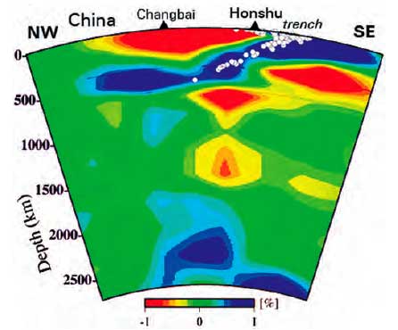
Figure 8. “It is now
well established that oceanic plates sink into
the lower mantle at subduction zones…” (image
from Zhao et al., 2004).
Summary
Global tomography has been used
to address the controversy of whether the upper
and lower mantles convect separately or as one.
However, the seismic tomographic method for imaging
the mantle suffers from several major problems
which preclude the results from simply showing
coherent structures, temperature distributions
or flow patterns. Transition zone boundary topography
often contradicts simple dynamic models based
on uncritical visual inspection of color cross-sections.
Tomography is useful for hypothesis testing and
for designing higher resolution experiments,
but it cannot directly and alone reveal mantle
dynamics. Waveform modeling, correlation statistics
and reflectivity studies are better suited for
gaining insight into that. High-resolution and
scattering studies give more information about
the homogeneity and heterogeneity of the mantle.
Resources:
words and pictures
The theoretical and observational
limitations of global tomography are well known
to experienced seismologists. Sometimes, however,
it is claimed that a new technique can resolve
features that were invisible to previous investigators,
even when fewer data are used. These claims are
discussed in the first reference below. The other
references discuss the limitations and artifacts
of tomography and give a number of models.
- de
Hoop, M.V. and van der Hilst, R.D., Reply
to comment by F. A. Dahlen and G. Nolet ‘On
sensitivity kernels for "wave-equation
transmission tomography", Geophys.
J. Int., 163, 952–955
doi: 10.1111/j.1365-246X.2005.02794.x GJI
Seismology, 2005.
- de Hoop, M.V., van der Hilst, R.D., and Shen,
P., Wave-equation reflection tomography: annihilators
and sensitivity kernels, Geophys. J. Int., 167,
1211-1214, 2006.
- Dziewonski,
A.M., Global seismic tomography: What we
really can say and what we make up, abstract,
Penrose Conference, Beyond the Plume Hypothesis,
Hveragerdi, Iceland, August 25th – 29th,
2003.
- Fukao, Y., Widiyantoro, S., and Obayashi,
M., Stagnant slabs in the upper and lower mantle
transition region, Rev. Geophys., 28,
291–323, 2001.
- Hamilton, W.B., Driving mechanism and 3-D
circulation of plate tectonics, in press in
J.W. Sears, T.A.Harms, and C.A. Evenchick,
editors, Whence the mountains? Inquiries
into the evolution of orogenic systems:
A volume in honor of Raymond A. Price: Geological
Society of America Special Paper 433, Chapter
1, 2007.
- Julian, B.R., Seismology:
The hunt for plumes, www.mantleplumes.org
webpage, 2004.
- Ritsema,
J., Global seismic maps, Web supplement,
2005.
- Ritsema, J., van Heijst, H.J., and Woodhouse,
J.H., Complex shearwave velocity structure
imaged beneath Africa and Iceland, Science, 286,
1925–1928, 1999.
- Shapiro, N.M., and Ritzwoller, M.H., Thermodynamic
constraints on seismic inversions, Geophys.
J. Int., 157, 1175–1188,
doi:10.1111/j.1365- 246X.2004.02254.x, 2004.
- Shearer, P.M., & Earle, P.S., The global
short-period wavefield modelled with a Monte
Carlo seismic phonon method, Geophys. J.
Int., 158, 1103–1117,
2004.
- Spakman, W., & Nolet, G., Imaging algorithms,
accuracy and resolution in delay time tomography,
in Mathematical Geophysics, Vlaar
et al. (eds.), Reidel, pp. 155–188, 1988.
- Thybo, H., & Perchuc, E., The seismic
8-degree discontinuity and partial melting
in the continental mantle, Science, 275,1626–1629,
1997.
- Tromp, J., Tape, C. & Liu, Q., Seismic
tomography, adjoint methods, time reversal
and banana-doughnut kernels, Geophys. J.
Int., 160, 195–216,
2005.
- van
der Hilst, R.D. & De Hoop, M.V., Banana-doughnut
kernels and mantle tomography, Geophys.
J. Int., 163, 956–961,
2005.
- van
der Hilst, R.D., & De Hoop, M.V., Reply
to comment by R. Montelli,, G. Nolet, and
F. A. Dahlen on "Banana-doughnut kernels
and mantle tomography", Geophys.
J. Int., 167, 1211-1214,
2006.
- Vasco, D. W., Johnson, L.R., Pulliam, R.J. & Earle,
P.S., Robust inversion of IASP91 travel time
residuals for mantle P and S velocity structure,
earthquake mislocations, and station corrections, J.
Geophys. Res., 99, 13,727–13,755,
1994.
The mapping of seismic velocity
into composition, lithology, temperature and flow
field is not straightforward, and may even be impossible.
The following references are useful in this regard.
- Anderson,
Don L., New Theory of the Earth 2nd
Edition; (ISBN-13: 9780521849593) DOI: 10.2277/0521849594.
408 pp, 2007.
- Ishii, M., & J. Tromp, J. Constraining
large-scale mantle heterogeneity using mantle
and inner-core sensitive modes, Physics
Earth Planet. Interiors, 146,
113–124, 2004.
- Lee, K.K.M. et al., Equations of state of
the high-pressure phases of a natural peridotite
and implications for the Earth’s lower
mantle, Earth Planet. Sci. Lett., 223,
381–393, 2004.
- Trampert, J., Vacher, P. & Vlaar, N.,
Sensitivities of seismic velocities to temperature,
pressure and composition in the lower mantle, Phys.
Earth Planet. Interiors, 124,
255–267, 2001.
- Trampert, J., Deschamps, F. Resovsky, J. & Yuen,
D., Probabalistic tomography maps chemical
heterogeneities throughout the lower mantle, Science, 306,
853–856, 2004.
The simplified interpretations
of color tomographic cross-sections that form the
basis of geochemical and geodynamic “standard
models” are based on just a few color-saturated
cross-sections. These have been superceded. If
one examines a large number of unsaturated maps
and cross-sections (see links below) one does not
get the impression of a one-layer pattern, or wholesale
sinking of slabs into the lower mantle. This is
confirmed by quantitative analysis and high-frequency
seismology. For example, convection modeling results
for layered mantle flow (Cizkova & Matyska,
2004) look more like tomographic cross-sections
than do whole-mantle convection simulations.
High-resolution seismology results
can be found on the web at the following sites;
http://www.sciencemag.org/cgi/data/1138074/DC1/1
http://epsc.wustl.edu/seismology/michael/CIG/workshop06/lectures/Levander_talk.pdf
http://www.ruf.rice.edu/~ctlee/2006LevanderLee.pdf
www.mantleplumes.org/
Baikal.html
http://www.mantleplumes.org/Iceland1.html
Search Goggle
Images with the following search strings;
Levander receiver-function imaging
receiver functions
receiver functions Iceland Yellowstone
Yellowstone receiver functions Dueker
References
-
Allegre, C.J. 1997, Limitation
on the mass exchange between the upper and
lower mantle: The evolving convection regime
of the Earth, Earth Planet. Sci. Lett., 150,
1–6.
-
Baig, P. & Dahlen, A.M.
2004, Traveltime biases in random media 1164
and the S-wave discrepancy, Geophys.
J. Int,. 158, 922–938,
1165 doi:10.1111/j.1365-246X.2004.02341.x.
-
Bercovici, D. & Karato,
S., 2003, Whole mantle convection and transition-zone
water filter, Nature, 425,
39-44.
-
-
-
Deuss, A., & J.H. Woodhouse,
2002, A systematic search for mantle discontinuities
using SS-precursors, Geophys.
Res. Lett., 29,10.1029/2002GL014768.
-
Fuchs, K., Tittgemeyer,
M., Ryberg, T., & Wenzel, F., 2002, Global
Significance of a Sub-Moho Boundary Layer (SMBL)
deduced from high-resolution seismic observations, Int.
Geol. Rev., 44, 671–685.
-
Fukao, Y., Widiyantoro,
S., & Obayashi, M., 2001, Stagnant slabs
in the upper and lower mantle transition region, Rev.
Geophys., 28, 291–323.
-
Gudmundsson, Ó.,
J.H. Davies, & R.W. Clayton, 1990, Stochastic
analysis of global travel-time data: Mantle
heterogeneity and errors in the ISC data, Geophys.
J. Int., 102, 25-43.
-
Helffrich, G.R. & Wood,
B.J., 2001, The Earth's mantle, Nature, 412,
501-507.
-
Ishii, M., & J. Tromp,
2004, Constraining large-scale mantle heterogeneity
using mantle and inner-core sensitive modes, Physics
Earth Planet. Interiors, 146,
113–124.
-
Kamber, B.S. & Collerson,
K.D. 1999, Origin of ocean island basalts:
a new model based on lead and helium isotope
systematics, J. Geophys. Res., 104,
479–91.
-
Kellogg, L.H. & Wasserburg,
G.J. 1990, The role of plumes in mantle helium
fluxes, Earth Planet. Sci. Lett., 99,
276–289.
-
Kellogg, L. H. et al. 1999,
Compositional stratification in the deep mantle, Science, 410,
1049– 1056.
-
Meyzen, C.M. et al. 2007,
Isotopic portrayal of the Earth's upper mantle
flow field, Nature, 447,
1069-1074.
-
Ricard, Y., Mattern, E. & Matas,
J. 2005, Synthetic tomographic images of slabs
from mineral physics, in, Earth's Deep
Interior: Structure, Composition, and Evolution,
van der Hilst, R.D., Bass, J.D., Matas, J.,
and Trampert, J. (Eds.), Geophysical Monograph,
American Geophysical Union, Washington, D.C., 160,
283-300.
-
Shapiro, N.M. & Ritzwoller,
M.H., 2004, Thermodynamic constraints on seismic
inversions, Geophys. J. Int., 157,
1175–1188, doi:10.1111/j.1365- 246X.2004.02254.x.
-
Shearer, P.M., & Earle,
P.S., 2004, The global short-period wavefield
modelled with a Monte Carlo seismic phonon
method, Geophys. J. Int., 158,
1103–1117.
-
Spakman, W. & Nolet,
G., 1988, Imaging algorithms, accuracy and
resolution in delay time tomography, in Mathematical
Geophysics, Vlaar et al. (eds.), Reidel,
pp. 155–188.
-
Spakman, W., S. Stein, R.D.
van der Hilst, & R. Wortel, 1989, Resolution
experiments for NW Pacific subduction zone
tomography, Geophys. Res. Lett., 16,
1097–1100.
-
-
Thybo, H., Nielsen, L., & Perchuc,
E., Sesimic scattering at the top of the mantle
transition zone, Earth Planet. Sci. Lett., 216,
259-269, 2003.
-
Trampert, J., Deschamps,
F. Resovsky, J. & Yuen, D. 2004, Probabalistic
tomography maps chemical heterogeneities throughout
the lower mantle, Science, 306,
853–856.
-
van der Hilst, R. D., Widiyantoro,
S. & Engdahl, E. R., 1997, Evidence of
deep mantle circulation from global tomography, Nature, 386,
578–584.
-
van der Hilst, R.D., 2004,
Changing views on Earth’s deep mantle, Science, 306,
817–818, 2004.
-
Vasco, D.W. & Johnson,
L.R., 1998, Whole Earth structure estimated
from seismic arrival times, J. Geophys.
Res., 103, 2633-2671.
-
Vasco, D.W., Johnson, L.R.,
Pulliam, R.J. & Earle, P.S., 1994, Robust
inversion of IASP91 travel time residuals for
mantle P and S velocity structure,
earthquake mislocations, and station corrections, J.
Geophys. Res., 99, 13,727–13,755.
-
Zhao, D., L. Jianshe & T.
Rongyu, 2004, Origin of the Changbai intra-plate
volcanism in northeast China: Evidence from
seismic tomography, Chinese Science Bulletin, 49,
1401-1408.
last updated
23rd September, 2007 |